mpg              wt              hp
 Min.   :10.40   Min.   :1.513   Min.   : 52.0
 1st Qu.:15.43   1st Qu.:2.581   1st Qu.: 96.5
 Median :19.20   Median :3.325   Median :123.0
 Mean   :20.09   Mean   :3.217   Mean   :146.7
 3rd Qu.:22.80   3rd Qu.:3.610   3rd Qu.:180.0
 Max.   :33.90   Max.   :5.424   Max.   :335.0
Correlations
Code
round(cor(mtcars[, c("mpg", "wt", "hp")]), 2)
      mpg    wt    hp
mpg  1.00 -0.87 -0.78
wt  -0.87  1.00  0.66
hp  -0.78  0.66  1.00
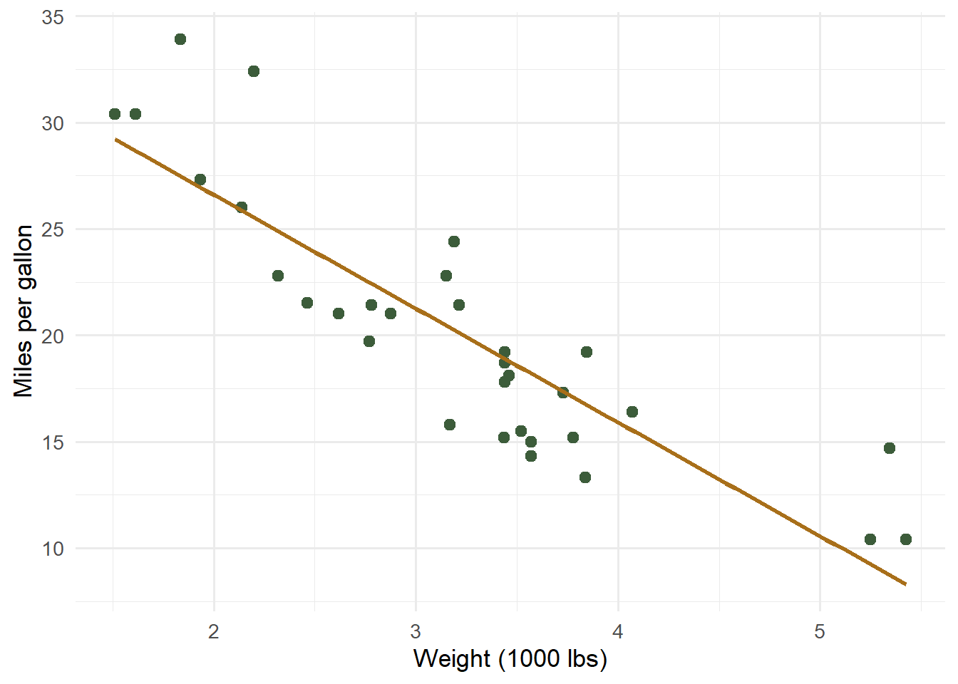
A plot
Code
library(ggplot2)ggplot(mtcars, aes(wt, mpg)) +geom_point(colour ="#3c5c3a", size =2.5) +geom_smooth(method ="lm", colour ="#a86f1a", se =FALSE) +labs(x ="Weight (1000 lbs)", y ="Miles per gallon") +theme_minimal(base_size =13)
Figure 1: Fuel economy falls as vehicle weight rises.
A simple model
Code
fit <-lm(mpg ~ wt + hp, data = mtcars)summary(fit)$coefficients
               Estimate Std. Error   t value     Pr(>|t|)
(Intercept) 37.22727012 1.59878754 23.284689 2.565459e-20
wt          -3.87783074 0.63273349 -6.128695 1.119647e-06
hp          -0.03177295 0.00902971 -3.518712 1.451229e-03
Wrapping up
If you can see the code, its output, and the plot above, Quarto and R are wired up correctly.